Summary: First in a quick(hopefully) series of posts on memory alignment in Java. This post introduces memory alignment, shows how to get memory aligned blocks, and offers an experiment and some results concerning unaligned memory performance.Since the first days of Java, one of the things you normally didn't need to worry about was memory. This was a good thing for all involved who cared little if some extra memory was used, where it was allocated and when will it be collected. It's one of the great things about Java really. On occasion however we do require a block of memory. A common cause for that is for doing IO, but more recently it has been used as a means to having off-heap memory which allows some great performance benefits to the right use case. Even more recently there has been talk of bringing back C-style
structs to Java, to give programmers better control over memory layout. Having stayed away from direct memory manipulation for long(or having never had to deal with it) you may want to have a read of the most excellent series of articles
"What Every Programmer Should Know About Memory" by Ulrich Drepper. I'll try and cover the required material as I go along.
Getting it straight
Memory alignment is mostly invisible to us when using Java, so you can be forgiven for scratching you head. Going back to basic
definitions here:
"A memory address a, is said to be n-byte aligned when n is a power of two and a is a multiple of nbytes.
A memory access is said to be aligned when the datum being accessed is n bytes long and the datum address is n-byte aligned. When a memory access is not aligned, it is said to be misaligned. Note that by definition byte memory accesses are always aligned."
In other words for n which is a power of 2:
boolean nAligned = (address%n) == 0;
Memory alignments of consequence are:
- Type alignment(1,2,4,8) - Certain CPUs require aligned access to memory and as such would get upset(atomicity loss) if you attempt misaligned access to your data. E.g. if you try to MOV a long to/from an address which is not 8-aligned.
- Cache line alignment(normally 64, can be 32/128/other) - The cache line is the atomic unit of transport between the main memory and the different CPU caches. As such packing relevant data to that alignment and to that punctuation can make a difference to your memory access performance. Other considerations are required here due to the rules of interaction between the CPU and the cache lines(false sharing, word tearing, atomicity)
- Page size alignment(normally 4096, can be configured by OS) - A page is the smallest chunk of memory transferable to an IO device. As such aligning your data to page size, and using the page size as your allocation unit can make a difference to interactions when writing to disk/network devices.
Memory allocated in the form of objects (anything produced by 'new') and primitives is always type aligned and I will not be looking much into it. If you want to know more about what the Java compiler make of you objects, this
excellent blog post should help.
As the title suggests I am more concerned with direct memory alignment. There are several ways to get direct memory access in Java, they boil down to 2 methods:
- JNI libraries managing memory --> not worried about those for the moment
- Direct/MappedByteBuffer/Unsafe which are all the same thing really. The Unsafe class is at the bottom of this gang and is the key to official and semi-official access to memory in Java.
The memory allocated via
Unsafe.allocatememory will be 8 byte aligned. Memory acquired via
ByteBuffer.allocateDirect will ultimately go through the
Unsafe.allocatememory but will differ in 2 important ways:
- ByteBuffer memory will be zero-ed out.
- Up until JDK6 direct byte buffers were page aligned at the cost of allocating an extra page of memory for every byte buffer allocated. If you allocated lots of direct byte buffers this got pretty expensive. People complained and as of JDK7 this is no longer the case. This means that direct ByteBuffer are now only 8 byte aligned.
- Less crucial, but convenient: memory allocated via ByteBuffer.allocateDirect is freed as part of the ByteBuffer object GC. This mechanism is only half comforting as it depends on the finalizer being called, and that is not much to depend on.
Allocating an aligned ByteBuffer
No point beating about the bush, you'll find it's very similar to how page alignment works/used to work for ByteBuffers, here's the code:
To summarize the above, you allocate as much extra memory as the required alignment to ensure you can position a large enough memory slice in the middle of it.
Comparing Aligned/Unaligned access performance
Now that we can have an aligned block of memory to play with, lets test drive some theories. I've used
Caliper as the benchmark framework for this post (it's great, I'll write a separate post on my experience/learning curve) and intend to convert previous experiments to use it when I have the time. The theories I wanted to test out in this post are:
Theorem I: Type aligned access provides better performance than unaligned access.
Theorem II: Memory access that spans 2 cache lines has far worse performance than aligned mid-cache line access.
Theorem III: Cache line access performance changes based on cache line location.
To test the above theorems I put together a small experiment/benchmark, with an algorithm as follows:
- Allocate a page aligned memory buffer of set sizes: 1,2,4,8,16,32,64,128.256,512,1024,2048 pages. Allocation time is not measured but done up front. The different sizes will highlight performance variance which stems from the cache hierarchy of sizes.
- We will write a single long per cache line (iterate through the whole memory block), then go back and read the written values (iterate through the whole memory block). There are usually 64 cache lines in a page (4096b/64b case), but we can only write 63 longs which will 'straddle' 2 lines, so the non-straddled offset will skip the first line to have the same number of operations.
- Repeat step 2 (2048/(size in pages)) times. The point is to do the same number of memory access operations per experiment.
Here is the code for the experiment:
Before moving on to the results please note that this test is very likely to yield different results on different hardware, so your mileage is very likely to vary. If you find the time to run the test on your own hardware I'd be very curious to compare notes. I used my laptop, which has an
i5-2540M processor(Sandy Bridge, dual core, hyper threaded, 2.6Ghz). The L1 Cache is 32K, L2 is 256K and L3 is 3M. This is important in the context of the changes in behaviour we would expect to see as the data set exceeds the capacity of each cache. Should you run this experiment on a machine with different cache allocations, expect your results to vary in accordance.
This experiment is demonstrating a very simple use case(read/write long). There is no attempt to enjoy the many features the CPU offers which may indeed stronger alignment than simple reading and writing. As such take the results to be limited in scope to this use case alone.
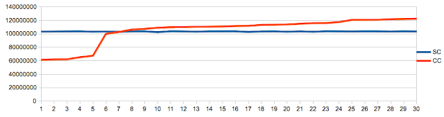
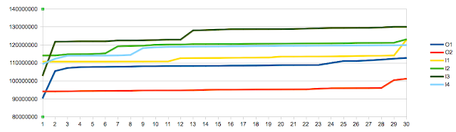
Finally, note that the charts reflect relative performance to offset 0 memory access. As the performance varied also as a function of memory buffer size I felt this helps highlight the difference in behaviour which is related to offset rather than size. The effect of the size of the memory buffer is reflected in this chart, showing time as function of size for offset 0:
The chart shows how the performance is determined by the cache the memory buffer fits into. The caches size in pages is 8 for L1, 64 for L2, and 768 for L3 which correspond to the steps(200us, 400us, 600us) we see above, with a final step into main memory(1500us). While not the topic at hand it is worth noting the effect a reduced data set size can have on your application performance, and by extension the importance of realistic data sets in benchmarking.
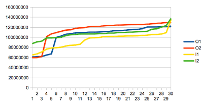
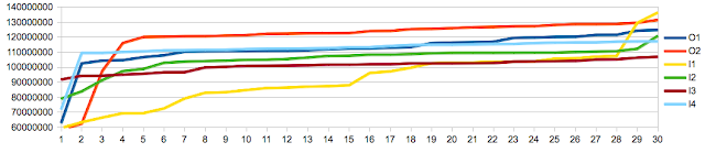
Theorem I: Type aligned access provides better performance than unaligned access - NOT ESTABLISHED (for this particular use case)
To test
Theorem I I set offset to values 0 to 7. Had a whirl and to my surprise found it made
no bloody difference! I double and triple checked and still no difference. Here's a chart reflecting the relative cost of memory access:
What seems odd is the difference in performance for the first 4 byte, which are significantly less performant then the rest for memory buffer sizes which fit in the L1 cache(32k = 4k * 8 = 8 pages). The rest show relatively little variation and for the larger sizes there is hardly any difference at all. I have been unable to verify the source of the performance difference...
What is this about? Why would Mr. Drepper and many others on the good web lie to me? As it turns out Intel in their wisdom have sorted this little nugget out for us recently with
Nehalem generation of CPUs, such that unaligned type access has no performance impact. This may not be the case on other non-Intel CPUs, or older Intel CPU. I ran the same experiment on my i5 laptop and my Core2 desktop, but could not see a significant difference. I have to confess I find this result a bit alarming given how it flies in the face of accepted good practice. A more careful read of
Intel's Performance Optimization Guide reveals the recommendation to align your type stands, but it is not clear what adverse effects it may have for the simple use case we have here. I will attempt to construct a benchmark aimed at uncovering those issues in a further post perhaps. For now it may comfort you to know that breaking the alignment rule seems to not be the big issue it once was on x86 processors. Note that behaviour on non-x86 processors may be wildly different.
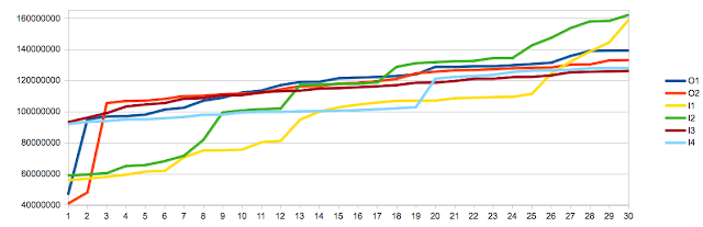
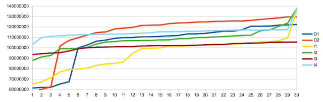
Theorem II: Memory access that spans 2 cache lines has far worse performance than aligned mid-cache line access - CONFIRMED
To test
Theorem II I set the offset to 60. The result was a significant increase in the run time of the experiment. The difference was far more pronounced on the Core2 (x3-6 the cost of normal access) then on the i5 (roughly x1.5 the cost of normal access), and we can look forward to it being less significant as time goes by. This result should be of interest to anybody using direct memory access as the penalty is quite pronounced. Here's a graph comparing offset 0,32 and 60:
The other side effect of cache line straddling is loss of update atomicity, which is a concern for anyone attempting concurrent direct access to memory. I will go back to the concurrent aspects of aligned/unaligned access in a later post.
Theorem III: Cache line access performance changes based on cache line location - NOT ESTABLISHED
This one is based on Mr. Dreppers article:
3.5.2 Critical Word Load
Memory is transferred from the main memory into the caches in blocks which are smaller than the cache line size. Today 64 bits are transferred at once and the cache line size is 64 or 128 bytes. This means 8 or 16 transfers per cache line are needed.
The DRAM chips can transfer those 64-bit blocks in burst mode. This can fill the cache line without any further commands from the memory controller and the possibly associated delays. If the processor prefetches cache lines this is probably the best way to operate.
If a program's cache access of the data or instruction caches misses (that means, it is a compulsory cache miss, because the data is used for the first time, or a capacity cache miss, because the limited cache size requires eviction of the cache line) the situation is different. The word inside the cache line which is required for the program to continue might not be the first word in the cache line. Even in burst mode and with double data rate transfer the individual 64-bit blocks arrive at noticeably different times. Each block arrives 4 CPU cycles or more later than the previous one. If the word the program needs to continue is the eighth of the cache line, the program has to wait an additional 30 cycles or more after the first word arrives
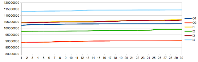
To test
Theorem III I set the offset values to the different type aligned locations on a cache line for a long: 0,8,16,24,32,40,48,56. My expectation here was to see slightly better performance for the 0 location as explained in Mr. Drepper's paper, with degrading performance as you get further from the begining of the cache line, at least for the large buffer sizes where data is always fetched from main memory. Here's the result:
The results surprised me. As long as the buffer fit in my L1 cache, writing/reading from the first 4 bytes was significantly more expensive than elsewhere on the line, as discussed in
Theorem I, but the other locations did not have measurable differences in cost. I pinged Martin Thompson which pointed me at the Critical Word First feature/optimization explained
here:
Critical word first takes advantage of the fact that the processor probably only wants a single word by signaling that it wants the missed word to appear first in the block. We receive the first word in the block (the one we actually need) and pass it on immediately to the CPU which continues execution. Again, the block continues to fill up in the "background".
I was unable to determine when exactly Intel introduced the feature to their CPU's, and I'm not sure which processors fail to supply it.
Conclusions/Takeaways
Of the 3 concerns stated, only cache line straddling proved to be a significant performance consideration. Cache line straddling impact is diminishing in later Intel processors, but is unlikely to disappear altogether. As such it should feature in the design of any direct memory access implementation and may be of interest to serializing/de-serializing code.
The other significant factor is memory buffer size, which is obvious when one considers the cache hierarchy. This should prompt us to make an effort towards more compact memory structures. In light of the negligible cost of type mis-alignment we may want to skip type alignment driven padding of structures when implementing off-heap memory stores.
Finally, this made me realize just how fast moving is the pace of development in hardware which invalidates past conventional wisdom/assumptions. So yet another piece of evidence validating the call to 'Measure, Measure, Measure' all things performance.
Running the benchmarks yourself
- Code is on GitHub
- Run 'ant run-unaligned-experiments'
- Wait... it takes a while to finish
- Send me the output?
To get the most deterministic results you should run the experiments pinned to a core which runs nothing else, that would reduce noise from other processes 'polluting' the cache.
Many thanks to
Martin,
Aleksey Shipilev and
Darach Ennis for proof reading and providing feedback on initial drafts, any errors found are completely their fault :-).


.jpg)